Introduction to digital signals
In a digital system, each signal is stored as a set of discrete samples that approximate the actual analog signal. If a signal is represented as a function of a continuous domain to a continuous co-domain, then digitization of the function consists of sampling the domain and quantizing the co-domain. This translates to a number of samples, each sample represented by a number of bits.
In an audio and video video system, sound and light are sampled and quantized based on a perceptual model of a human ear and eye respectively. Those digital signals can then be used to recreate sound and light a human being will identify as identical to the original signals.
An audio signal is characterized as air pressure on the eardrum through time. Its digital representation consists of quantized pressure levels through time samples. An audio signal is spatially located by placing a number of speakers around the listener. A channel is associated to each speaker and a specific channel is dedicated for low frequencies. Hence, you will usually see notation like 5.1, meaning five normal channels and one low frequency effect channel.
A video signal is characterized as light intensity and wavelength detected by each photoreceptor cell in the retina through time. Typically, a digital video signal is a time-sequence of still frames where each frame is spatially divided into pixels. A progressive signal samples a frame at each clock. None-the-less because of the way earlier television sets were working, video signals are still often today sampled as an interlaced signal. A interlaced signal samples odd lines at each other clock and even lines on the alternate tick. Hence, 720p at 25Hz indicates a progressive signal where 25 full frames are sampled every second while 1024i at 50Hz indicates an interlaced signal where 25 odd-lines and 25 even-lines fields are sampled per second. The human eye is such that most humanly visible colors can be accurately modeled with a combination of red, green and blue wavelengths. Color video systems thus use a quantization of red, green and blue intensities.
| Audio | Video | |
|---|---|---|
| sampling | frequency |
pixel resolution and frames per second |
| quantization | amplitude | intensity |
| examples |
CD audio 16-bit 44.1kHz |
DVD Video 24-bit 640x480x25 (640 horizontal, 480 vertical, 25 frames/sec.) |
| High-definition | ||
|
up to 7.1 96kHz at 24-bit. |
1920x1024i at 60Hz |
Samples representation
Audio and video digital signals can be stored and exchanged between many systems from different vendors. It is much better each bit of each sample is interpreted identically on each system; that avoids annoying effects such as blowing up speakers for example.
The byte-order, sign and interpretation of a sample's bits need to be clearly specified for stored media data. This is usually done in international standards that get settle after a few "standard wars". Those standards also detail how quantization is done such that reconstruction of the signal can be done accurately.
Most audio input and output devices work with Pulse Code Modulation. That is each sample is interpreted as an integer being the actual magnitude of the signal at a point in time. As an example, the CD format defined in IEC 60908 (aka Red Book) encodes samples as signed 16-bit little-endian linear PCM.
Audio signals can be isolated. You might listen to a bass track alone, then add the guitar and it will not change the sound of the bass. This is not the case with video systems. If you remove the green component from a color picture, that picture will look very different from the original full color picture. You will loose all yellows. The interpretation of each pixel thus includes the color model.
A common pixel representation uses 24 bits interpreted as three 8-bit unsigned integer for Red, Green and Blue intensities. Television systems commonly uses three 8-bit unsigned integers, one for intensity and two chroma components known as YCbCr. YCbCr is a linear derivation of RGB where Y can be used to drive a black and white television set.
As a human eye is more sensitive to intensity than chroma, it is often the case to store a chroma pair per two or four Y values, hence reducing bandwidth requirements. YCbCr is sometimes loosely referred as YUV and the previous representations as YUV444 (one chroma pair per intensity), YUV422 (one chroma pair per two intensities) and YUV420 (one chroma pair per four intensities).
| Audio | Video |
|---|---|
| 16-bit PCM |
8-bit RGB 8-bit YUV420 |
Multi-channel samples can be stored in different ways. A planar representation stores channels sequentially while an interleaved representation stores samples sequencialy.
Audio and video systems
Performance is linked to the intrinsic characteristics of the algorithm, the compiled code and the specifics of the hardware platform.
Audio and Video Algorithms
There are thousands of audio and video algorithms and DSP processing remains a very active research field. Fortunately most algorithms can be categorized based on their computation characteristics. This helps predict compute-load and evaluate system-on-chip when building new consumer products.
Re-sampling
As seen previously, sampling is critical to model a signal accurately and so it is no surprise that re-sampling is a major function of any media solutions. A few examples of re-sampling includes use cases such as following.
A 5.1 signal that need to be rendered on a stereo system has to be down-mixed from 5 to 2 channels. A high-fidelity microphone samples at 96kHz and the final signal needs to be stored on an audio CD at 44.1kHz.
A DVD rendered on an high-definition television set will have to be up-scaled to fit the entire screen while a picture-in-picture will require to downscale the original signal. Interlaced video signals will have to be de-interlaced before rendered onto progressive scan LCD screens.
Filtering
Filters are used to smooth artifacts introduced by the sampling process, enhance signals and provide special effects. As examples, equalizers can be found in any audio systems while convolution filters are standard in video processing.
Transformation
Domain transformation is key to many signal analysis and compression because it permits extraction of correlations inside a signal. From far the most widely used domain transforms in digital processing are Fast Fourier Transforms, related Discrete Cosine Transforms, and their inverses. Wavelet transforms have properties very useful for compression and are also used in newer systems.
Rotations, color conversions and other linear algebra transforms are also often present in many systems.
Bit-stream parsing
Bit-stream parsing is a major part of audio and video compression for two reasons: multiplexing and variable length coders.
In order to deliver audio and video signals, both signals are multiplexed into a single stream. The receiver parses the incoming bit-stream, de-multiplex each sub-stream and routes each signal to the appropriate device.
After filtering and transformations, digital signals are compressed using derivatives of standard compression tools such as Huffman, arithmetic and other variable length coders.
Bit-stream parsing is an interesting and challenging problem for system designers. Whereas other digital signal processing (DSP) algorithms are inherently parallel, thus benefit from more hardware resources, variable length coding is inherently sequential. Each bit of the a variable length encoded block need to be decoded before the next bit in the block can be in turn decoded. With a Context Adaptive Arithmetic Coder (CABAC) such as the one used in H264, most blocks cannot be decoded in parallel either because the surrounding (i.e. top and left) blocks are used to drive the arithmetic coder.
Processors and system architecture
A few basic concepts of general-purpose processors help understand some of the observed behavior and thus what and how to optimize whole systems.
caches
Memory capacity and processing power have increased and continue to increase rapidly. The speed and bandwidth of the underlying bus communication has not followed the pace. Transferring bytes between different part of the systems often becomes a bottleneck and the main reason for caches popping-up all around the system.
Roughly, level one caches are small memory buffers tightly coupled to the processor that hold a duplicate of parts of slower bigger memory. The expectation is that caching reduces bus bandwidth requirements and hides bus latency. Data moves in and out of caches onto the memory bus as a result of the processor issuing load and store instructions.
Hence analyzing the data access pattern of the DSP algorithms executed is a major requirement for performance analysis and optimization. Buses, caches and data movements have to be the focus of attention for system designers.
Details of cache architectures can be found elsewhere. For our purpose here, caches are associative maps of addresses to lines with two characteristics of major importance: cache size and cache line size.
Since a cache is orders of magnitude smaller than memory, at some point lines need to be evicted from the cache and more useful data brought in. The cache size will thus dictates the working set, or the amount of data that can be used and re-used without having to move data back and forth to memory.
For that reason, a signal will most times be split into processing packets with a full packet designed to fit in the cache. The processing pipeline is then organized around packets instead of algorithms. This optimization technique works until the machine code to execute for each packet becomes large enough and generates unwanted cache evictions.
Caches have a line-oriented interface to the memory subsystem. Every load whose address misses in the cache will trigger a fetch of an entire cache line. With a cache line of 64 bytes, loading one byte whose address misses will fetch 64 bytes from memory into the cache.
The base and size of data arrays will have most times to be adjusted, i.e. aligned, to increase cache efficiency. For example, it is common for a picture to be defined with a width and an implementation stride.
With these few examples, one can see that optimization requires a deep understanding of access patterns, data layout in memory and their interactions with specific caches implementation.
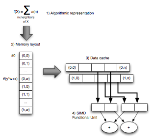
compute kernels
The properties of signals composition translates into the digital world as arithmetic in either [0,1[ or [-1,1[ domains. Values in those domains are represented in processors with a finite number of bits interpreted either as a fixed-point or floating-point number. Two signals are composed with a sequence of multiplication and addition operators and the final result is then saturated to fit in the unit domain.
First, either in fixed-point or floating-point, each computation introduces rounding errors. To compensate those effects, so the compute kernel uses a greater bit depth than the bit depth of the input and output signals.
Second, each compute kernel is usually executed in loops over samples and channels. This regularity makes it possible to execute the same instruction stream on multiple data at the same time. Processors implement Single-Instruction Multiple-Data (SIMD) operations for that purpose.
Outside signal composition and analysis, audio and video systems contain variations of general compression algorithms. Branches, bit extraction, bit insertion and table look-up make up most of the processor operations used in bit parsing. The increasing complexity of variable-length coders, especially the latest ones such as the Context Adaptive Binary Arithmetic Coder (CABAC), creates pressure on system designers to find creative solutions to the complex problems involved.
Useful Resources
- Digital Video and HDTV, Algorithms and Interfaces - Charles Poynton
- Computer Architecture, a quantitative approach - John L. Hennessy and David A. Patterson